
Author: René Sultan
AI telemetry tells us which models our agents use and what they cost, but not what we are paying them to do. We built a semantic layer that turns agent traces into the record of purpose, outcome, and cost needed for ROI attribution.
The pipeline builds this semantic layer from agent traces. It combines related sessions into complete agent runs, then separates each run into work items. A work item is a distinct objective the agent pursued. Each work item records its goal and outcome, along with labels for the kind of work, product or platform domain, and technical surface involved. We link it to the run’s model spend, owner, team, and repository. Over three weeks, the system analyzed roughly 200,000 agent runs and identified roughly 250,000 work items.
Before this, our telemetry showed which models ran, how many tokens they used, and what they cost. That gave us a view of spend based on how AI was consumed. To reason about ROI, we needed a view of what our agents produced: the objective, the result, the team, the product, and the system involved. The semantic layer gives us a clear path to ROI attribution. By connecting these records to product and business outcomes, we can move from knowing what AI cost to evaluating what it returned.
Ramp Inspect
We started with Inspect, Ramp’s internal background coding agent. Each Inspect session runs in a remote sandbox with a full development environment and access to the tools and context available to a Ramp engineer. This lets Inspect read code, query internal data, make API requests, implement changes, and verify them through tests and live previews.
As of August 2026, 75% of all PRs merged at Ramp came from Inspect sessions, and Inspect had crossed one million total sessions. Its use extends beyond direct coding. Engineers, designers, and product managers collaborate in Inspect sessions, while more than 200 internal agents run on the platform for workflows including code review, incident response, data analysis, and customer feedback. That scale and variety made Inspect the natural place to start.
The traces already contained the information needed to understand this range of work. Each trace records the user’s request and the agent’s execution: its messages, tool calls, code changes, tests, and outcome. A person could read a trace and understand what the agent was asked to do, what it did, and how the work ended. Our challenge was to turn that manual reading into consistent analysis across hundreds of thousands of sessions.
Reconstructing a complete run
A request to Inspect does not always stay within one session. Here, a session means one Inspect execution. Inspect can open child sessions to investigate another repository, work on part of the request in parallel, or continue related work in a new session. Those sessions can open child sessions of their own.
One request involved a workflow that analyzes a business’s recent bank activity and upcoming payments to recommend how much money it should add to a connected bank account to cover the next 30 days. This example is based on a real request, but names and repository identifiers have been changed.
The user request began with:
If you look at funding recommendation runs it seems like the web app always dispatches two runs for some reason... can you double check if this is a bug?
Inspect split the work into this session family:
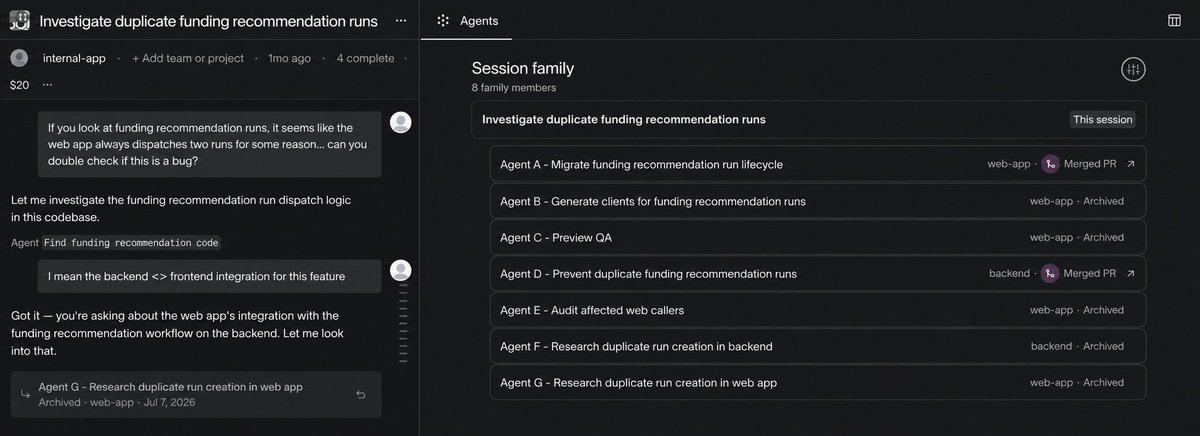
The root session coordinated the request and handled the internal-app changes. Two child sessions investigated the frontend and backend. A session in the backend repository implemented the fix and opened another session to audit the affected web callers. A separate web session migrated the frontend and opened sessions for preview QA and generated API clients.
Together, the eight sessions used roughly 5.6 million tokens, exchanged 1,100 messages, made 960 tool calls, and cost $93. The root contained only about one-fifth of that spend. Both merged PRs came from child sessions.
We therefore made reconstruction the first step in the pipeline. The reconstruction process starts from the root, follows every child and continuation, waits for all of them to finish, and combines their traces into one record. We call the root session and its linked child and continuation sessions a complete run. Only then does the extraction model interpret the consolidated work.
Extracting work items from a complete run
Once reconstruction finishes, the extraction model reads the complete run and extracts work items. We define a work item as the basic unit of agentic work: one objective and one outcome.
The extraction model’s main input is a chronological trace of the root session and every child session, including their messages, tool calls, commands, file changes, tests, and final outcomes. We also pass facts derived from the trace: whether reconstruction was complete, how many messages and tool calls it contained, which files appeared most often, which tools were used, and whether the run changed code, opened a PR, failed, or crossed repositories.
For the funding recommendation example, the extraction model received one record containing all eight sessions shown above. It could see the original request, the frontend and backend investigations, the backend fix, the frontend migration, the QA sessions, and both merged PRs together.
The difficult part was deciding where one work item ended and another began. Investigating, editing, testing, and explaining are often phases of the same objective. Treating every phase or child session as a separate item would overcount the work, but one run can also pursue several objectives that should remain separate.
The funding recommendation run shows this distinction. The investigation identified the cause of the bug. The backend change fixed it. The frontend migration adapted the affected clients to the new API. The extraction model kept these as three work items because each had a separate objective and outcome. It treated QA and code generation as supporting steps, not independent work items.
We encoded that distinction in the prompt:
Extract work items only for distinct user or business objectives. Do not split normal implementation phases like investigate, edit, test, and explain into separate work items unless they serve distinct objectives. A child session that pursues a distinct objective is usually its own work item; a child that simply continues the parent’s objective usually is not.
The extraction model returns a structured response at two levels. One describes the complete run. The other contains a detailed record for each work item.
At the run level, the response included:
In total, the extraction model identified three work items:
- Root cause analysis of duplicate funding recommendation runs. Determine whether the duplicate runs originated in the frontend or backend. The investigation traced them to concurrent backend requests creating the same run.
- Prevent duplicate run creation in the backend. Change the backend so concurrent requests reuse the same run instead of creating duplicates. The resulting PR prevented duplicate runs.
- Update frontend orchestration to the new API. Update the affected frontend clients to create the run once, then make read-only requests using the returned run ID. This work produced a second merged PR.
Each work item points back to the evidence that supports it, including the relevant sessions, files, tools, and artifacts. This lets us check the extraction against the original trace.
Across roughly 200,000 analyzed runs, 17% contained more than one work item. Of those multi-item runs, 61% took place entirely within a single session. The inverse was also true: 30% of runs that expanded into several linked sessions only represented one work item. There was no one-to-one mapping between Inspect sessions and work items. Additionally, the 17% of multi-item runs accounted for 58% of model spend.
At this point, we were able to decompose any complete run into its component work items, but we still needed a shared taxonomy to compare hundreds of thousands of runs.
Describing each work item
We ran the labeling model separately for each extracted work item. It received the structured work-item record shown above and a summary of the complete run. The run summary supplied the surrounding context, while the prompt instructed the labeling model to label only the selected work item.
We asked the labeling model to describe each item in three ways:
- What its work type was
- Which domain it supported: the product or internal platform
- Which technical area it touched
We specified what each label should describe, but did not specify fixed values that the labeling model could return. We deliberately did not give the labeling model a predefined taxonomy or set of labels at this stage. Doing so would have built our assumptions into the output and forced unfamiliar work into the closest available category.
Instead, the labeling model wrote each label in its own words, allowing it to capture uses of Inspect we had not anticipated.
The central instruction was:
Label the work item, not the whole session, while preserving session context. Use free-form, natural-language labels. Do not force the work item into a preset taxonomy or menu of category values.
The response also described the item’s intent, workflow, outcome, missing context, and supporting evidence. Six fields captured the labels we later used to build shared categories.
For the root-cause analysis from the funding recommendation run, the labeling model returned:
Together, these fields described the work type, domain, and technical area.
The three work items from the funding recommendation example received these free-form labels:
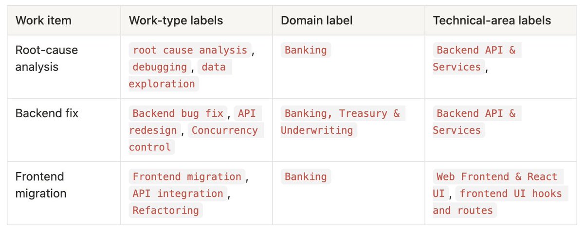
These were the labeling model’s descriptions, not the shared categories shown later in the attribution dashboard. At this stage, variation was useful. It allowed the labeling model to preserve distinctions we had not anticipated, use specific language when the evidence supported it, and say when an area was not visible instead of guessing.
Next, we wanted a consistent way to group the resulting labels. Equivalent concepts could appear under different names or at different levels of specificity, such as Banking and Banking, Treasury & Underwriting. To group and compare work across hundreds of thousands of runs, we needed to turn that vocabulary into a shared taxonomy.
Building a shared taxonomy
The labeling model described investigative work at different levels of specificity, using labels such as debugging, root cause analysis, and production investigation. Across three weeks, it wrote more than 1.4 million labels for roughly 250,000 work items. One work item could receive several labels describing its work type, domain, and technical area. After normalizing those labels, more than 100,000 unique values remained.
To build the first taxonomy, we used the taxonomy model to group a set of observed labels into shared categories. For each label, the input included:
- The label itself.
- What it described: work type, domain, or technical area.
- How often it appeared.
- Examples of work items that used it.
We asked the taxonomy model to group labels that expressed the same idea while preserving distinctions that remained useful for analysis:
Merge obvious spelling, casing, punctuation, and synonym variants. Do not over-merge labels that would hide meaning a manager, product owner, or Inspect owner would care about.
The taxonomy model returned separate categories for work type, domain, and technical area. Each category had a name, a definition, the observed labels grouped under it, and examples of the work those labels described.
The first published taxonomy contained 30 categories:
- 10 work types
- 11 domains
- 9 technical areas
For the funding recommendation run, the shared categories were:
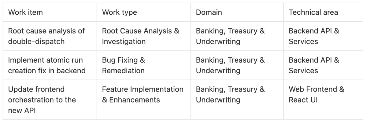
The labels written by the labeling model preserved what was specific about each work item, while the shared categories gave us a consistent way to compare work across runs and attribute spend by work type, domain, and technical area.
Compressing agent traces
After the initial three-week analysis, cost became the next constraint. To keep running the pipeline at company scale, we needed to identify what drove that cost and reduce it without changing the work items or categories it produced.
To do this, we compressed each extraction input to the information the extraction model needed. Each extraction call sent the extraction model an average of roughly 76,000 input tokens. About 74,000 of them, or 98%, came from the agent trace. That made the trace the clearest place to reduce cost.
We began by measuring what the traces contained:
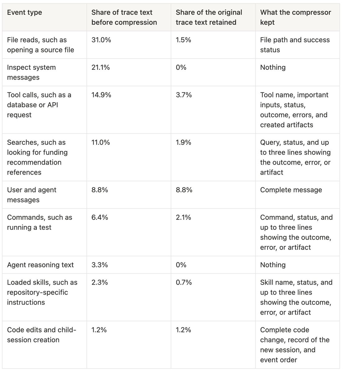
The largest share was file reads. Inspect stored the complete contents of every file it opened, even though the extraction model usually needed only the file path and whether the read succeeded.
For example, a file-read event could contain:
The compressor reduced it to:
For searches, commands, and tool calls, it kept the action and the lines that recorded what happened. A long test log, for example, became:
When the same long result appeared more than once, the compressor kept the first copy and replaced later copies with a reference:
We kept user and agent messages, code edits, and child-session records in full. Those events carried the request, the changes made, and the structure of the complete run. We removed agent reasoning text and Inspect system messages because they described how Inspect operated rather than what the user requested or what the run produced.
We then tested whether compression changed what the pipeline reported. Because LLM inference is not perfectly deterministic, repeated analyses of identical input can produce slightly different labels. We first ran the uncompressed extraction repeatedly on identical inputs to measure that normal run-to-run variation. Then we compressed roughly 4,000 historical traces and repeated the extraction. Across work type, domain, and technical area, the differences between the compressed and uncompressed results remained within the variation we had already observed between uncompressed reruns.
We measured the token reduction across traces ranging from fewer than 25,000 characters to more than 1.2 million. Compression reduced the average trace from roughly 74,000 to 19,000 tokens, a 74% reduction, while preserving the conversations, code changes, and outcomes used to understand the run.
Making the attribution queryable in Snowflake
Finance, product, and engineering teams needed to combine this attribution with the data they already used to measure spend, ownership, and outcomes. We therefore published the results in Snowflake at two levels:
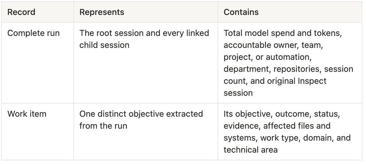
Every work item points back to the complete run that produced it. This connects model spend to several levels of context at once: the accountable owner, which project and repositories were involved, what the agent was trying to achieve, what it did, and how the work ended.
Spend is measured once for the complete run. For each category view, we distribute that total evenly across the distinct categories represented in the run. Applying the same rule to every run keeps total spend fixed while allowing it to be compared by work type, domain, and technical area.
The funding recommendation example would no longer appear only as a $93 line item under the broad Software Engineering department. We could see that the spend supported the funding recommendation workflow within Banking, Treasury & Underwriting. We could trace it across internal-app, backend, and web-app, separate the investigation from the backend fix and frontend migration, identify the accountable owner, and see that the work produced two merged PRs.
The same structure supports much more specific questions across Ramp. A user of Router could isolate spend associated with the Router project, separate work on routing behavior from evaluations, backend integrations, and prompt or skill changes, then see which people or automations initiated those runs and how each one ended.
Inspect also powers more than 200 internal agents for workflows such as code review, incident response, and data analysis. The attribution lets us analyze these automated runs with the same detail as work initiated directly by a person. For a code-review agent, we can move from total spend categorized as Code Review to the repository and pull request it reviewed, the product or system that code supported, the findings it produced, and whether those findings led to a code change.
Finance could move from asking how much Engineering spent on Inspect to questions such as:
- How much did the Router project spend on evaluations and routing changes?
- Which products generated the most Inspect spend on debugging?
- Which repositories and accountable owners were behind that spend?
- How much code-review spend supported Banking rather than internal developer tooling?
- Which expensive runs produced merged changes, completed investigations, or no shipped result?
These records changed how we could analyze AI spend. Instead of organizing it only by model, token count, and department, we could organize it around the project, objective, outcome, accountable owner, product, and technical system involved.
This is the missing layer between AI spend and AI ROI. Once spend carries the purpose and result of the work behind it, we can compare it with the product, engineering, and business outcomes Ramp already measures and ask the question that matters: did the result justify what we spent?
Productizing AI spend attribution
We productized the attribution by turning the Snowflake records into a company-wide view of where Inspect spend went, which objectives and products it supported, who owned the work, and how each run ended.
The view is designed to move from aggregate spend to its source. A user can begin with all Inspect activity across Ramp, then narrow it by time, department, accountable owner, repository, work type, domain, or technical area.
Filtering to one accountable owner shows their total model spend, number of complete runs, and average spend per run. The same view shows their top work types, domains, technical areas, and repositories, followed by the runs that contributed to those totals.
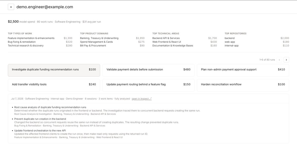
The funding recommendation example shows this path from aggregate to source. Selecting Root Cause Analysis & Investigation reveals the $93 run behind part of that spend. The user can see the investigation that found the backend race condition, the backend change that fixed it, and the frontend migration that followed. The run also links back to Inspect, where its complete session family and original traces remain available.
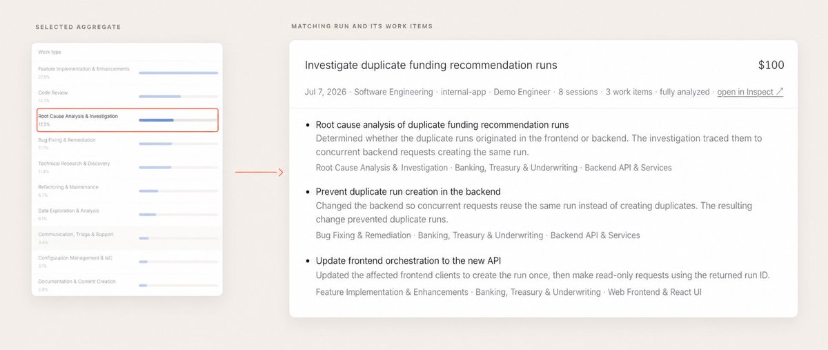
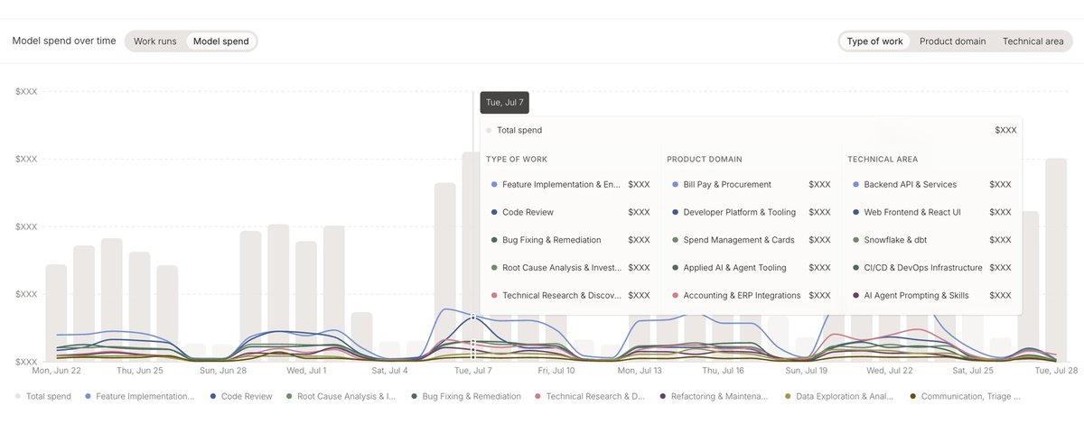
A category total therefore remains connected to the work that produced it. Finance can start with the total Inspect model spend attributed to Bug Fixing & Remediation across Ramp, narrow it to a particular product, owner, or repository, then inspect the runs and fixes behind that amount. A product or engineering owner can start from their project, compare where its AI spend went, and examine how the most expensive runs ended.
Productizing the attribution also gave Ramp a shared way to interpret the data. Finance, product, and engineering teams use the same definitions of work type, domain, technical area, ownership, and outcome. Company leaders can compare spend across the organization, while the people closest to the work can verify the objectives, results, code changes, and original Inspect sessions behind the numbers.
With the attribution available as a company-wide product, we could see how Inspect was actually being used across Ramp and what the company was receiving for that spend.
The path from AI Spend to AI ROI
Measuring AI ROI cannot start with tokens or model calls. It has to start with the objective an agent was asked to pursue and the outcome it helped produce. Cost becomes meaningful when we can connect it to purpose: what the work was meant to achieve, who it supported, and what changed as a result.
That is the context our semantic layer creates. It connects model spend to the objectives behind the work, how the work ended, its accountable owner and team, and the products and technical systems involved. At Ramp, we can now see the purpose behind our AI spend at company scale and trace any total back to the underlying work.
From there, we can connect AI spend to the product, engineering, and business measures Ramp already uses to evaluate investments. Did the agents working on Router help the team ship faster? Did spending on Banking investigations make the product more reliable? Did AI reduce the manual work required to keep Finance’s product economics models up to date? These are judgments finance and business leaders already make about people, software, and projects. The semantic layer gives them the record they need to make those judgments about AI.
The next generation of AI cost management will not stop at measuring what AI costs. It will show what the investment was for, what it produced, and whether it was worth it. This semantic layer is our foundation for building that future at Ramp. If you’re interested in using this product, email us at veeral@ramp.com and rene.sultan@ramp.com to be added to the alpha.
Want to keep up with our next AI experiments? Subscribe here and follow us on @RampLabs. We’re also hiring across roles at Ramp.